Interactive Simulator Usage Guide
The Python script interactiveSim.py uses the Linux native application of Meshtastic to simulate multiple instances of the device software. These instances communicate using TCP via the script, simulating the LoRa chip. The simulator forwards messages from the sender to all nodes within range, based on their simulated positions and the selected pathloss model (see Pathloss Model). Note: Packet collisions are not yet simulated.
Usage
-
Clone or download the repository and navigate to the Meshtasticator folder.
-
(Optional) Create a virtual environment.
-
Install dependencies:
pip install -r requirements.txt
The simulator runs the Linux native application of Meshtastic firmware. You can use either PlatformIO or Docker to run the firmware:
Using PlatformIO
Select 'native' and click 'build.' Locate the generated binary file, likely in firmware/.pio/build/native/.
Copy the program file to the directory where you'll run the Python script, or provide the path as an argument with -p:
python3 interactiveSim.py 3 -p /home/User/Meshtastic-device/.pio/build/native/program
Using Docker
The simulator pulls a Docker image that builds the latest Meshtastic firmware.
Ensure the Docker SDK for Python is installed:
pip3 install docker
Make sure the Docker daemon or Desktop app is running. Use the -d argument to launch the simulator:
python3 interactiveSim.py 3 -d
Running the Simulator
To run the interactive simulator:
python3 interactiveSim.py [nrNodes] [-p <full-path-to-program>]
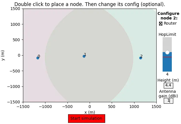
nrNodes(optional): Number of instances to launch. Each instance opens a terminal and a TCP port (starting at 4403).- If you provide the number of nodes, they will be randomly placed; otherwise, you can manually place nodes on a plot.
- After placing nodes, you can configure their role,
hopLimit, height (elevation), and antenna gain. Configurations are saved automatically.
Commands During Simulation
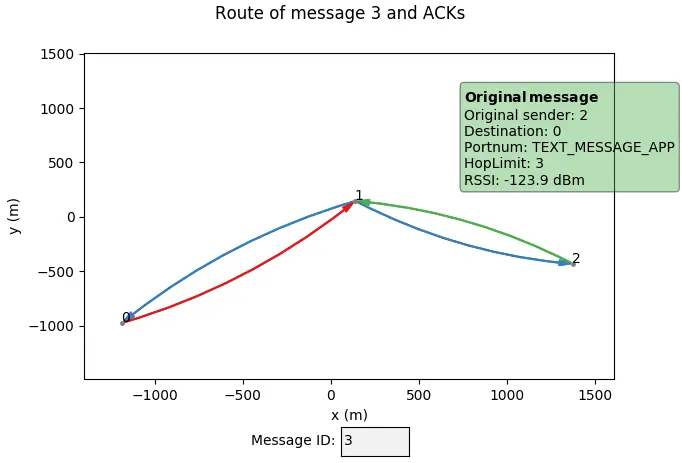
Once the simulation starts, you can issue commands (or use a predefined script) to send messages between nodes. Use plot to visualize message routes and airtime statistics:
- Enter a message ID to see its route.
- Hover over arcs for information and click to remove the overlay.
- Two graphs display channel utilization (one-minute window) and airtime usage (hourly window) for each node.
List of Commands
broadcast <fromNode> <txt>: Send a broadcast from node fromNode with text txt.DM <fromNode> <toNode> <txt>: Send a Direct Message from node fromNode to node toNode with text txt.traceroute <fromNode> <toNode>: Send a traceroute request from node fromNode to node toNode.reqPos <fromNode> <toNode>: Send a position request from node fromNode to node toNode.ping <fromNode> <toNode>: Send ping from node fromNode to node toNode.remove <id>: Remove node id from the current simulation.nodes <id0> [id1, etc.]: Show the node list as seen by node(s) id0, id1, etc.plot: Plot the routes of messages sent and airtime statistics.exit: Exit the simulator without plotting routes.
Usage with Script
Modify the try clause in interactiveSim.py to predefine messages. Run the simulator with the -s argument:
python3 interactiveSim.py 3 -s
- After nodes exchange NodeInfo, they will begin sending messages.
- Close the simulation manually with
Ctrl+Cor wait for the timeout.
Tips and Tricks
-
Speeding Up NodeInfo Exchange:
Disable certain modules by removingnew NodeInfoModule()fromsrc/modules/Modules.cppin the firmware. -
Saving and Reloading Configurations:
After a simulation, node configurations are saved. You can rerun the same scenario with:python3 interactiveSim.py --from-fileModify the
out/nodeConfig.yamlfile to adjust configurations before reloading. -
Using the Python CLI:
You can call functions from the Node class viasim.getNodeById(<id>)ininteractiveSim.py. Example:node.setURL('<YOUR_URL>')
Pathloss Model
The simulator estimates signal propagation using a pathloss model. This is an approximation of the physical environment, so it may not be 100% accurate. The available models are:
- 0: Log-distance model
- 1: Okumura-Hata model (small/medium cities)
- 2: Okumura-Hata model (metropolitan areas)
- 3: Okumura-Hata model (suburban environments)
- 4: Okumura-Hata model (rural areas)
- 5: 3GPP model (suburban macro-cell)
- 6: 3GPP model (metropolitan macro-cell)
You can modify the pathloss model and area configuration in lib/config.py. LoRa settings remain at their Meshtastic defaults unless customized during node placement.